Finite Difference Gradients in Neuronal Circuits
Using Pytorch to compute gradients explicitly in circuits of realistic complex neuronal models, especially those with very complex internal connections, can be very computationally expensive. Furthermore, I think that issues such as numerical stability will become significant because of all the multiplications over every timestep, among other factors. One idea is to compute gradients using something different to backpropogation. In particular, I tried out using finite difference methods instead, which, as far as I can tell online, is not a particularly well-researched idea, especially in terms of actual applications.
The idea is simple, suppose we have a function: $$f: A \rightarrow B, x \mapsto y.$$ Then, to measure the gradient of \(f\) with respect to \(x\), we can approximate it using a small perturbation \(\Delta x\): $$\frac{\partial f}{\partial x} \approx \frac{f(x + \Delta x) - f(x)}{\Delta x}.$$ Now, suppose we have some network of neurons, for example a fully connected network of 5 neurons with weights:
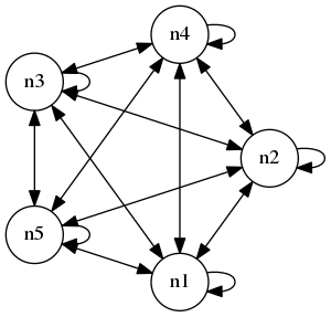
Suppose each neuron has some internal state \(V\) and some associated output \(a\) (these are dependent on time but I will not mention that for now). Let us denote the weighted output of all neurons as \(z\). So, if we put the weights into a 5 by 5 matrix \(W\), then $$z = W a$$ I think in most real networks, the matrix \(W\) will be sparse. Now, suppose we have some function \(f: \mathbb{R}^5 \rightarrow \mathbb{R}\) that quantifies the output into a single scalar. Suppose we want to measure how the weights affect \(f(z) = f(W a)\). At first, it might seem that we need to measure all weights' influence on this quantity. However, as in traditional backpropogation, we can actually just measure the influence of the weighted input \(z\) on \(f\) and then "interpolate" to the individual weights by an outer product. In particular, by the chain rule, $$D_{_W} f(z) = (\nabla f(z))^T \cdot D_{_W} z = (\nabla f(z))^T \cdot a^T,$$ so we just measure the left gradient \(\nabla f(z)\) (which, before the transpose, is a row vector), then take an outer product with the unweighted output \(a\).
Next, we compute the gradient using finite-difference methods. In particular, we compute the individual partial derivatives \(\partial f / \partial z_i\) which compose the gradient. This is done by the following: $$\frac{\partial f}{\partial z_i} \approx \frac{f(z_i + \Delta z_i) + f(z_i)}{\Delta z_i}.$$ The incremement \(\Delta z_i\) should be small, and I'm not sure what is a good criterion for choosing it exactly. My mind turns to grid computations and other stuff when I see the rule above but I haven't fleshed out those ideas yet.
In summary: to compute the total derivative \(D_{_W} f\), we first approximate \(\nabla f(z)\) as above, then we take an outer product with \(a\).
Network of Coupled Oscillators
I wanted to use a simple oscillator model to try out these ideas in a more specific application and see how we do. The Van der Pol oscillator is a simple 2D oscillator model given by:
$$x' = y$$
$$y' = \mu (1 - x^2) y - x,$$
for some parameter \(\mu\). With this simple model we can get some cool plots easily. For example, here is a plot of the phase space for a grid of initial conditions from -5 to 5 demonstrating that all the states reach a stable cycle:
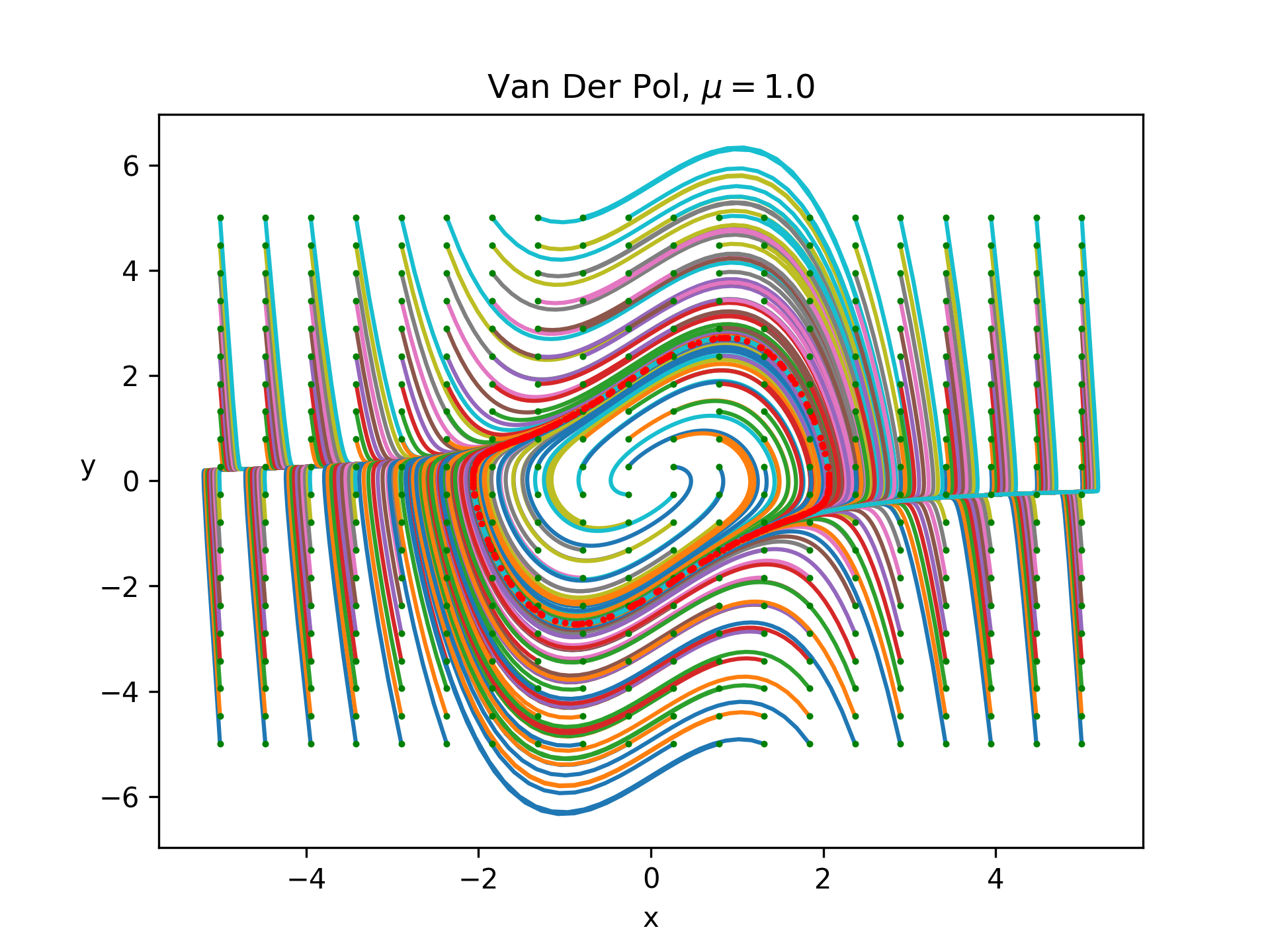 The green dot denotes the initial condition and the red denotes the final conditions and everything was simulated for 30 time units with a timestep of 0.03.
Let's add some more complexity by considering a network of coupled Van Der Pol oscillators. In particular, a quick google search linked me to this paper which looks at the dynamics of two coupled oscillators. In their equations, they add a new direct term to \(x'\) and \(y'\) based on the difference between these quantities and the mean of these quantities throughout the network. These terms are scaled by some fixed constants \(\epsilon_A, \epsilon_B\) and added to the original ODE. I decided to first set \(\epsilon_B\) to zero, so we only have input through the \(x\) variable. Next, I introduced weights, so that, instead of looking at the input average to a neuron, we look at the weighted input average based on the particular neuron's weights. With these changes the vectorized system now looks like:
$$x' = y + \epsilon (z - x)$$
$$y' = \mu (1 - x^2) y - x,$$
where \(z\) is the weighted quantitiy
$$z = W x.$$
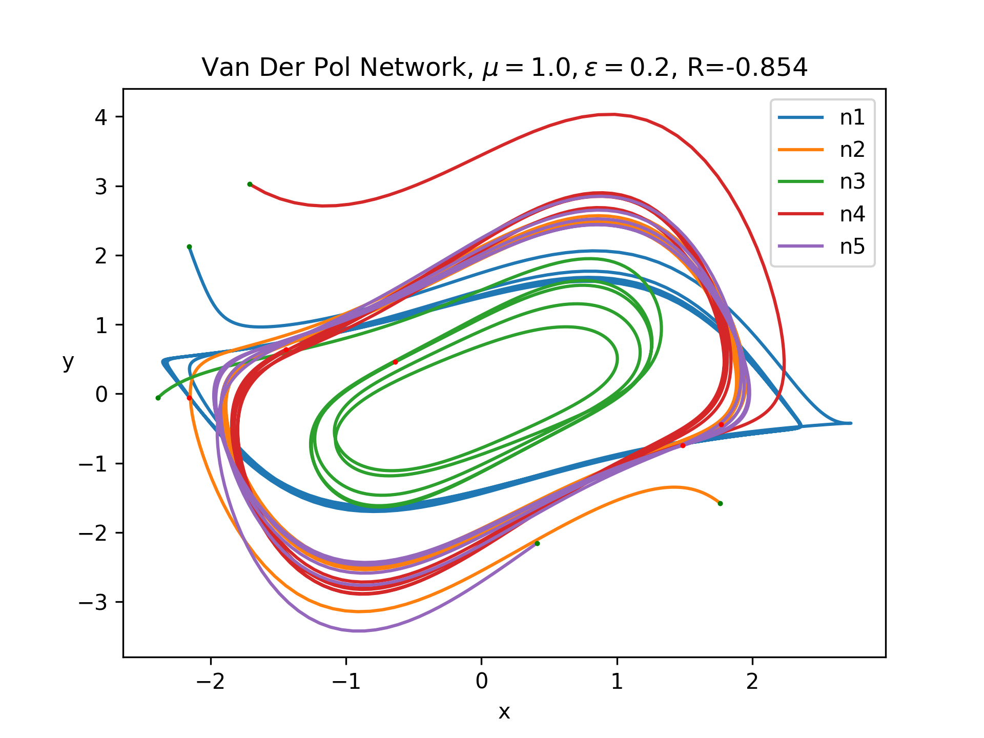
Let's look at the behavior with a network of 5 fully connected neurons with random normal weights and random normal initial conditions with a standard deviation of 2, as in the graph at the top of this page. Below is a plot of some sample trajectories:
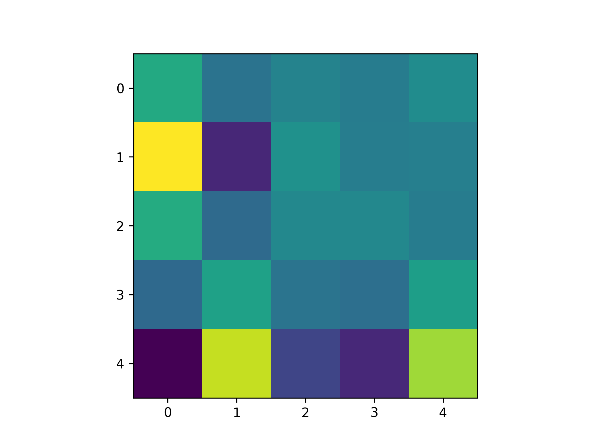
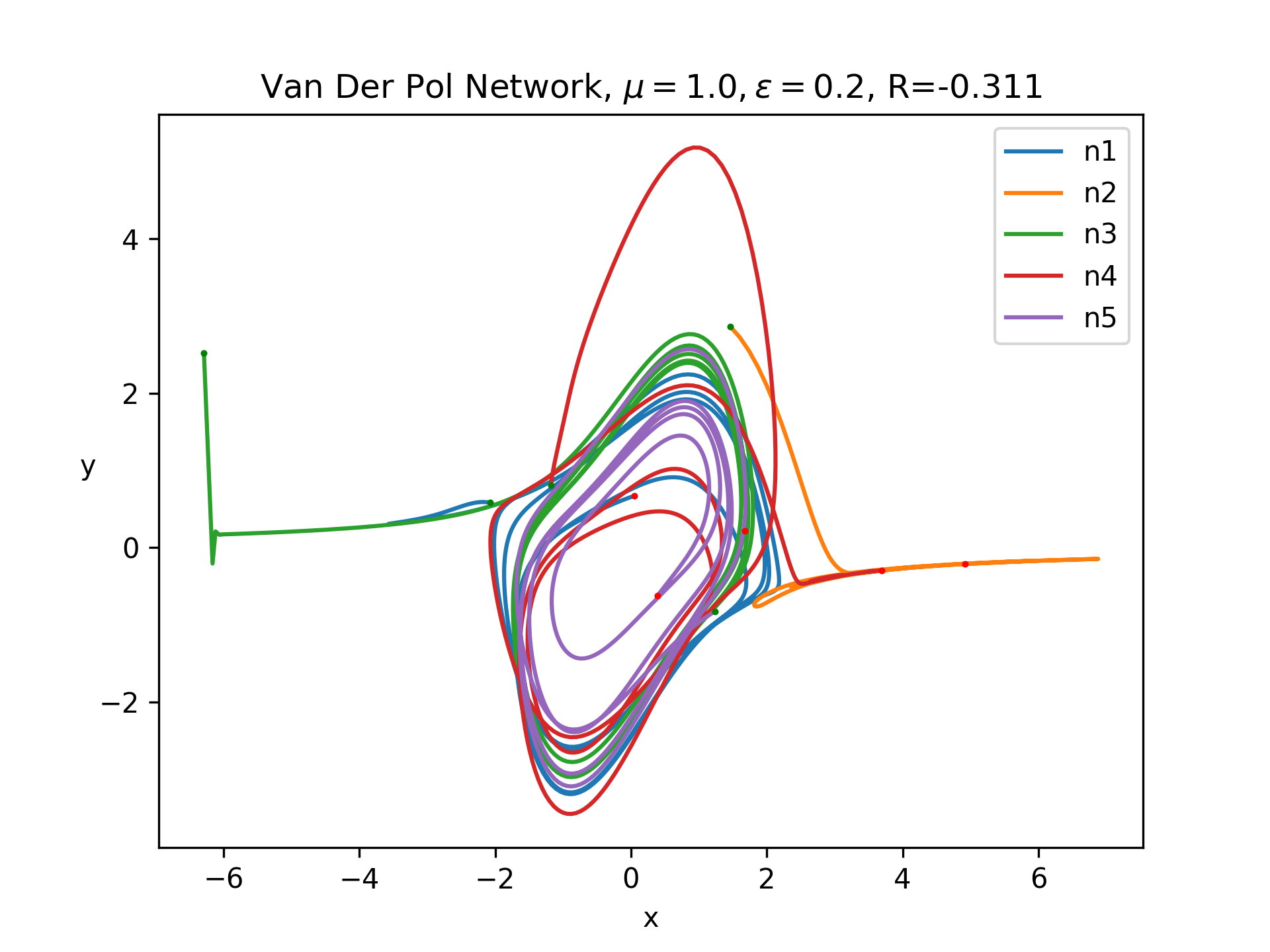 We need some way to convert this network to a quantifiable single scalar quantity. In real machine learning tasks, this is a loss function. In our case, I am just screwing around, so let's come up with something on the fly. Inspired by the paper I linked above, let's try use the Pearson correlation coefficient. This is motivated by the idea that taking the gradient of this quantity with respect to weights should tell us how the weights affect correlation in the network, assuming we have simulated for a sufficiently long time period. One detail is that Pearson correlation only considers two signals. Thus, I just measured the correlation between the first two neurons. Then, I measured the gradients using the methods above. Here is the resulting matrix:
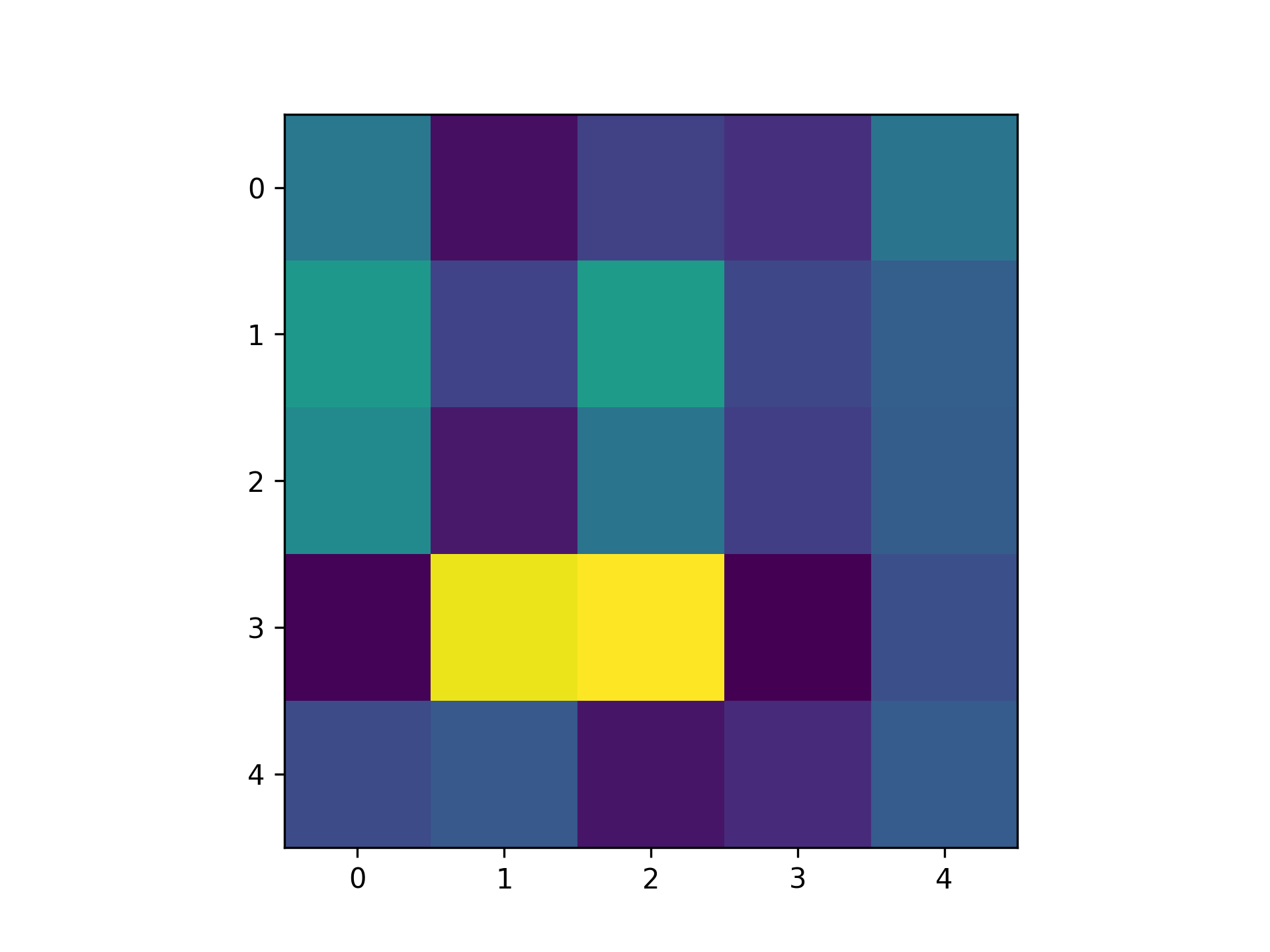 Here's another example: